Pattern of trade for the US and China

Key points:

• The decomposition of time series of imports and exports of the US and China (mainland) and the comparison of the results allows us to note a lot of interesting features not clearly visible from basic visual comparison
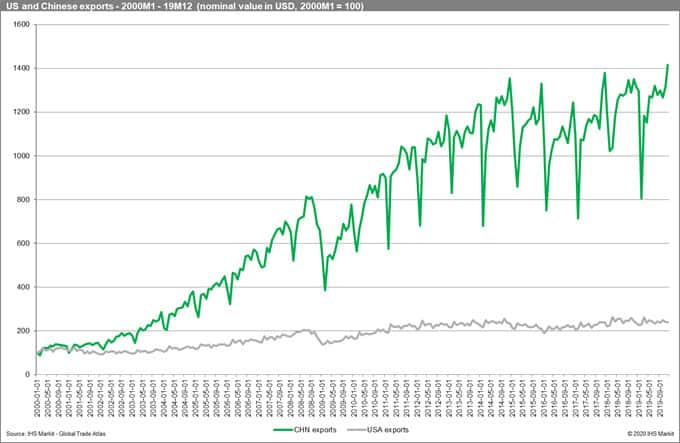
• In the analyzed period (2000M1 - 2019M12) Chinese exports have grown by around 14 times with the US only more than doubling
• We observe one structural break for both countries from July 2008 to February 2009 - the result of the global financial crisis followed by a rapid recovery
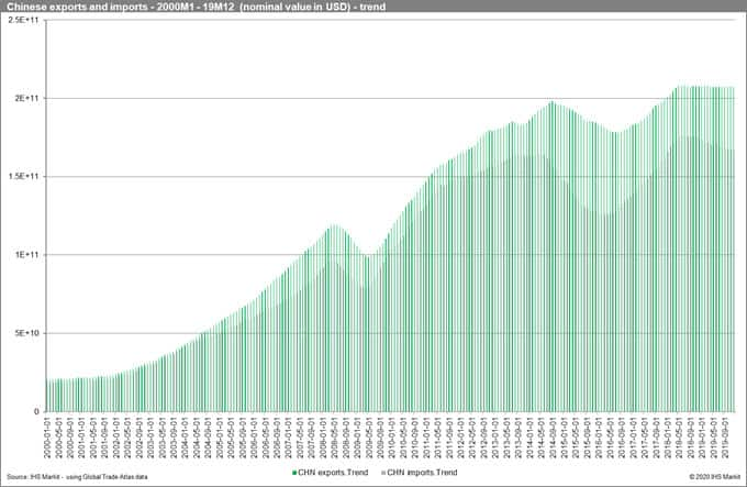
• The trends for US and Chinese exports and imports are non-linear
• Both US and Chinese exports and imports show significant seasonality; the seasonal component is stronger for China than for the US
• For US exports, we have two peaks in March and October. For imports, there is one clear peak in October. Generally, US imports' seasonal component is decreasing from October to February and then more or less grows steadily to October (with the lowest value in February). The exports behave differently - they fall from October (a peak) but start to recover a month ahead in January with a strong rise in activity in March (the first peak) and then oscillate with peaks in June, August, and October
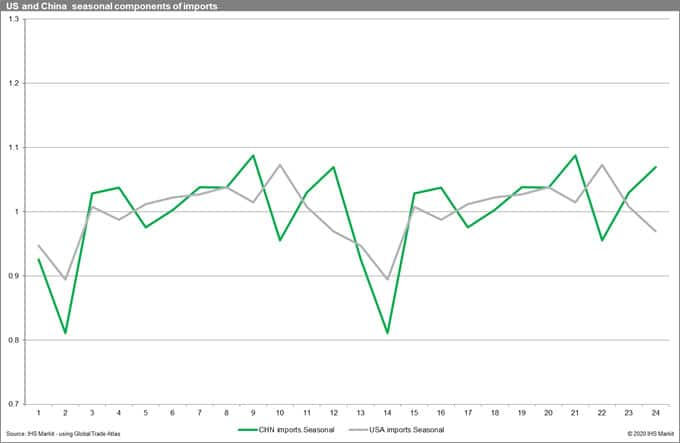
• For Chinese exports we observe two peaks in September and December. For imports we see three peaks in activity in March-April, September and December. Both imports and exports of China are falling in January - February (with February the lowest point in activity within a year)
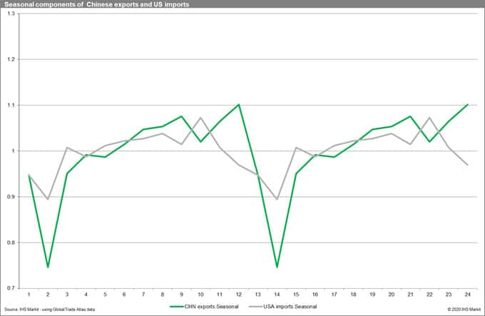
• Interestingly the seasonal component of Chinese exports coincides well with US imports; it is significantly lower vice versa
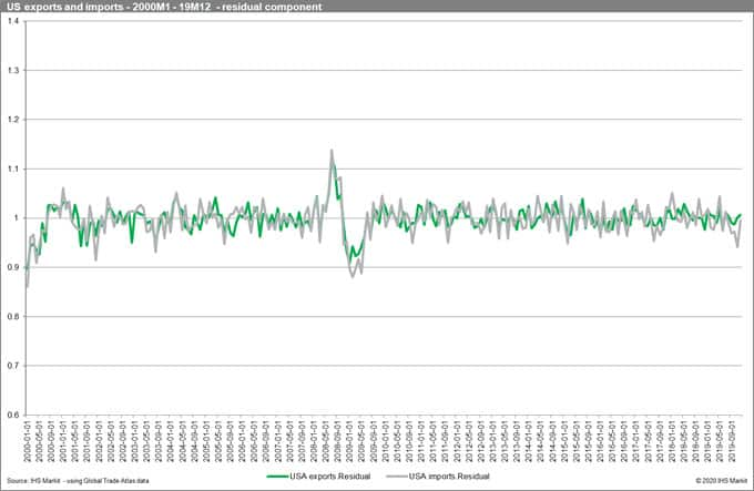
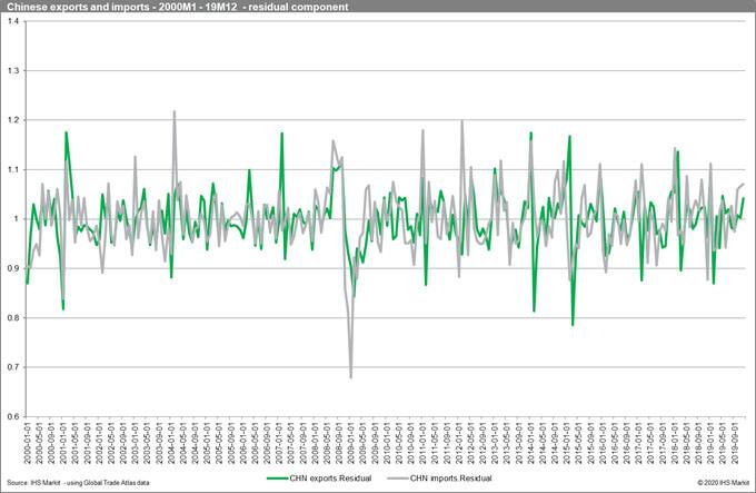
• The residual component shows a similar level of disturbances, however, once again the amplitude of shocks is significantly higher for China

Introduction

Using the monthly data on trade from the Global Trade Atlas we have analyzed the pattern of trade of the two largest economies of the world - the US and China (mainland). The period under analysis was January 2000 (2000M1) - December 2019 (2019M12). This gives us 480 observations. We utilize data on the nominal value of exports and imports in USD treating the time series for exports and imports independently.

Decomposition of time series

Time series decomposition involves thinking of a time series as a combination of level, trend, seasonality, and noise (residual) components. Decomposition provides a useful model for thinking about time series and enhances our understanding of time series analysis and forecasting.

The present decomposition has been performed in Python using the seasonal decompose module from the statsmodels library. The naive form of decomposition can accommodate both additive and multiplicative type of models.

The overall evolution of trade

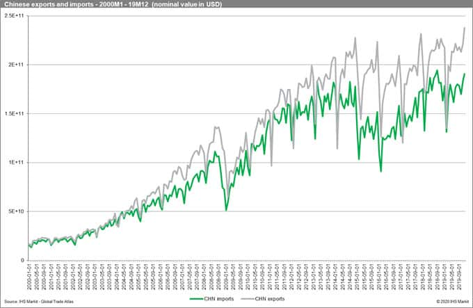
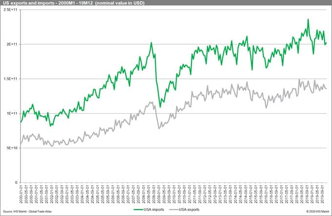
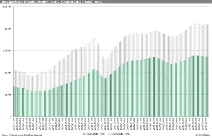
Reviewing the line plots above, it suggests the existence of trends, potentially nonlinear for China. Seasonality is evident and the amplitude of the cycles appears to be increasing. It suggests the multiplicative version of the model.

A simple visual analysis allows us to draw several conclusions. Chinese exports and imports have clearly caught up with the value of US exports and imports over the analyzed period. This reflects the unprecedented growth of the Chinese economy and gradual convergence. The US has a permanent deficit in their trade relations, while China enjoys a permanent surplus - with its size changing within the year - the surplus decreases in size or even becomes a deficit only in February and/in March. Moreover, we observe one structural break for both countries from July 2008 to February 2009 - the result of the Lehman Brothers bankruptcy and the following global financial crisis. Furthermore, we observe a return to the preceding trends in late 2009 - 2010.

In order to be able to more directly compare the time series for the US and China in the chart beneath, we relativize their respective exports by setting the 2000M1 to 100. Chinese exports have grown by around 14 times with US only more than doubling. The amplitude of changes within a year is significantly higher for China. The US series is much more stable. Both show, however, a seasonal component.

Trend components

In the first stage we will compare the trend components of our decomposition. Both for the US and China, the trends are nonlinear and different. They are more similar for exports and imports for the same country. For the US we can spot three major falls in the trend - 2000-2001, 2008-2009 and 2014-2015. For China, the major breaks are in 2008-2009, 2014-2016 and for imports since mid-2018. The two common breaks are 2008-2009 and 2014-15 (16).

Seasonal components

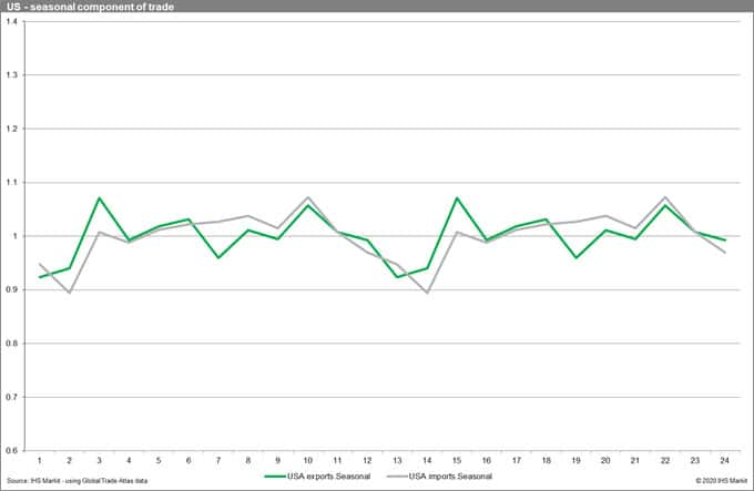
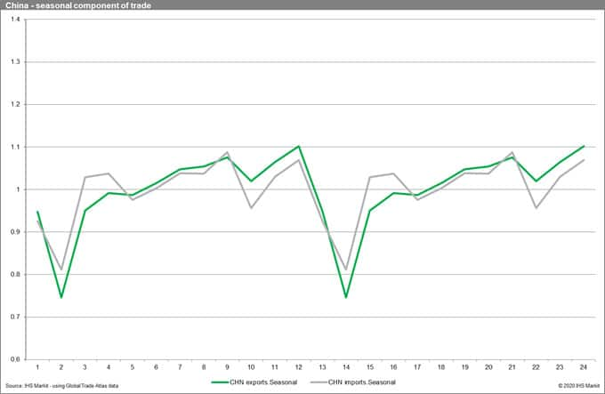
The US seasonal component of trade shows a lower amplitude than Chinese (both charts beneath utilize the same scale). The seasonal components for exports and imports for both countries are similar.

For US exports we have two peaks in March and October. For imports, there is one clear peak in October. Generally, US imports' seasonal component is decreasing from October to February and then more or less grows steadily to October (with the lowest value in February). The exports behave differently - they fall from October (a peak) but start to recover a month ahead in January with a strong rise in activity in March (the first peaks), and then oscillate with peaks in June, August and October.

For Chinese exports, we observe two peaks in September and December. For imports, we see three peaks in activity in March-April, September and December. Both imports and exports of China are falling in January - February (with February the lowest point in activity within a year).

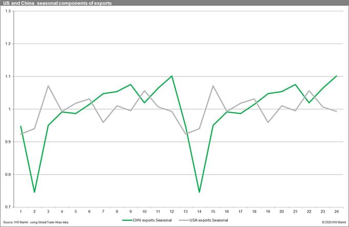
The differences in seasonal components of US and China exports and imports described above become more evident visually if they are more directly compared. Overall the correlation is higher for imports than for exports. More interestingly, the correlation of seasonal components is the highest between seasonal components of US imports and Chinese exports. It is much less evident the other way around.

Residual components

Finally, it is interesting to compare the noise or the random variation in the analyzed series which is non-systematic and cannot be directly modeled. This can contain important information on the disturbances or shocks to the economic system, for instance, major black-swans or major policy shifts.

Once again, we can observe that US trade in comparison to Chinese is much more stable. The number of disturbances is similar; however, the magnitude is visibly higher for China. The direct comparison of the residual components also allows us to clearly see that 2008-2009 was the most significant disturbance to the two analyzed economies.

This column is based on data from IHS Markit Global Trade Atlas.